How to write a simple photographic mosaicker
Today we'll learn how to write a simple photographic mosaicker! You've probably seen those large pixelated images that are composed of tiny irrelevant images, like a portrait of Obama that comprises tiny cat pictures. These are known as photographic mosaics. Here I'll describe a very simple approach to creating such a mosaic, using nearest neighbor search and the CIFAR-10 dataset.

Image of a seagull comprising tiny hexagons. No, we’re not recreating this, but something similar!
A little backstory: last semester, I was the teaching assistant for CS534 Computational Photography here at Wisconsin, and at the end of the semester I was asked, by a commissioner who projected a silhouette of a bat onto the Wisconsin night sky, to come up with new assignment ideas. This idea of a photographic mosaicker didn't make the cut because it didn't fit in our existing syllabus, but the effect is so strong and the approach is so simple that I thought I'd share it here!
You'll need
- An input image. This is a fairly large color image that you want the mosaic to look like. Let the size of the image be H×W.
- A library of tiny images. We use a subset of the CIFAR-10 dataset. Let the number of tiny images be Nt.
- MATLAB with the statistics toolbox, or any language with a nearest neighbor implementation.
Steps
- Shrink your tiny images to an appropriate size D×D. If D is large, you can recognize the content of the tiny images within the mosaic and that looks impressive, but the mosaic becomes coarse and starts looking less like the input image; if D is small, the mosaic reconstructs the input image well, but you can't tell what's in the tiny images, which kind of defeats the purpose of such a mosaic. You've got to strike a balance.
- Shave off the borders of the input image, so that the height and width are each multiples of D, otherwise you can't create the mosaic effect at the 'leftover' portions of the input image.
- Unroll the input image patches and the tiny images, into the observation matrix X and query matrix Y, respectively. X should be a Nt×D2 matrix since each D×D tiny image is unrolled into a vector of length D2. Similarly, you should cut up the H×W input image into many non-overlapping D×D patches, unrolled to produce a (HW⁄D2)×D2 matrix.
- Run 1-nearest-neighbors! Here we're just finding the most similar (in Euclidean distance between raw pixel intensities) tiny image for every patch in the input image.
- Replace every patch in the input image with its nearest neighbor found in the previous step. Depending on your actual implementation, you probably have to roll the tiny images back into squares in this step.
- And... we're done!
Results
Below we use a scene of Madison's beautiful Lake Mendota as the input image. You can't take such a picture now, not just because the lake is frozen now, but also because Memorial Union is closed off for renovations. But when it's accessible Lake Mendota is gorgeous. I digress.
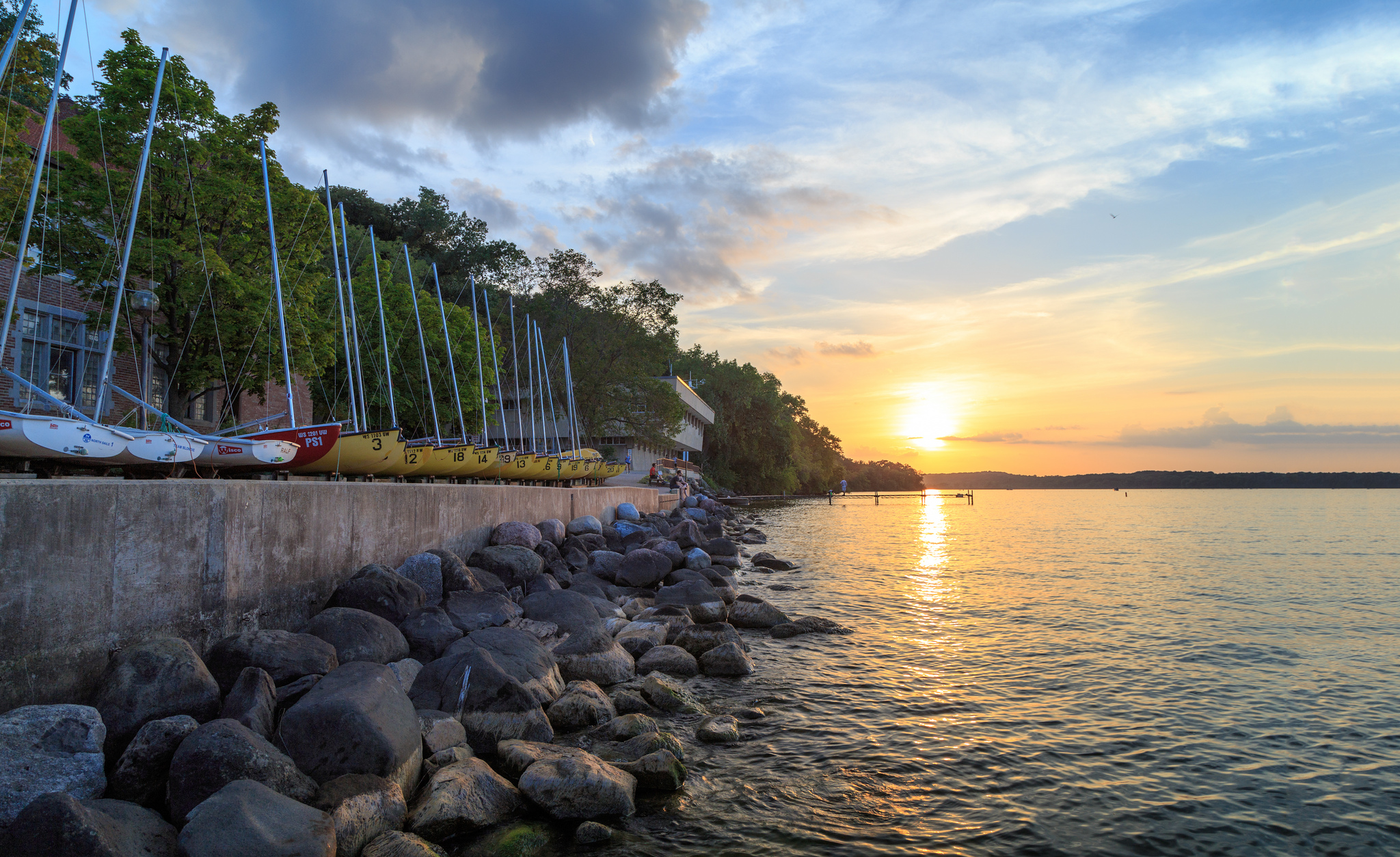 Input image of Lake Mendota, WI Madison
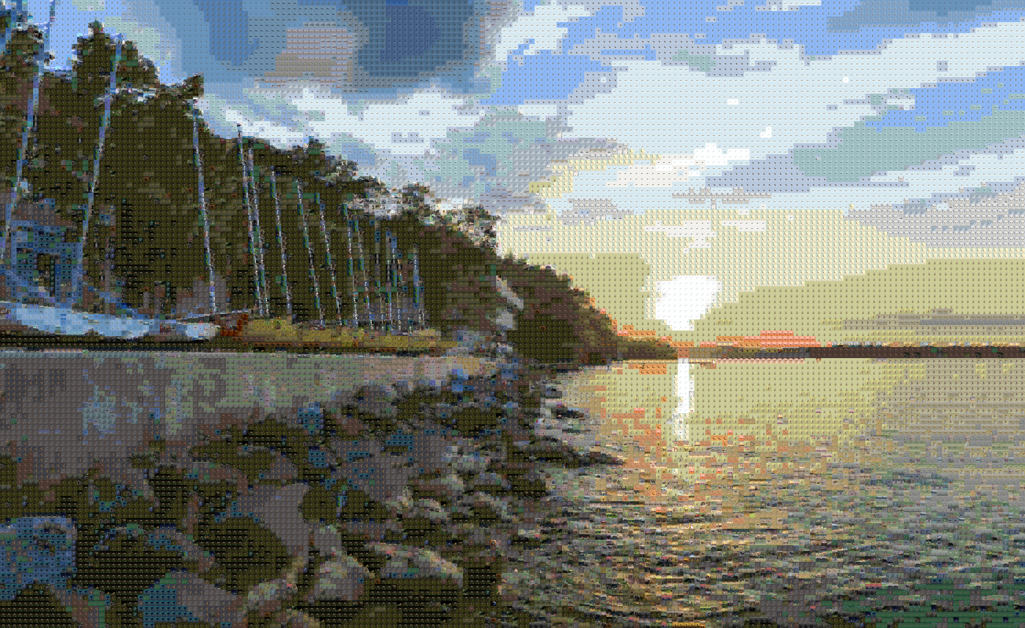 Image mosaic of Lake Mendota comprising CIFAR-10 images
The effect is really good for such a simple approach! Notice that we used raw pixel intensities to find nearest neighbors, which is probably a bad feature representation since we really don't care about the spatial distribution of colors within the tiny image - we just need the colors between the input image patch and its tiny image to match. Something like a histogram of intensities along with Earthmover's distance would be more effective but complicates the code slightly. Here we overcame the limitation of using raw pixel intensities by shrinking the tiny images to be really tiny, so that we get a decent distribution of observations in feature space. The drawback, as mentioned, is that you can barely make out what the tiny images are within the mosaic.
Hope this was helpful!
(A gist of the above algorithm can be found here)